plotting package
This module contains mainly a class Mapfigure, which makes it easier to create Basemap plot and add a method to plots trajectories on top of it.
Examples
First let’s load the class:
>>> from dypy.plotting import Mapfigure
Then prepare a map you have two main options:
with a domain definition:
>>> domain = [5, 10, 45, 47]
>>> m = Mapfigure(domain=domain)
Or with lon, lat coordinates:
>>> m = Mapfigure(lon=lon, lat=lat)
In this case, the domain is based on the boundary values of the lon, lat arrays.
The next step is to plot data on the map:
>>> m.contourf(lon, lat, data)
or, if m was prepared using option 2:
>>> m.contourf(m.x, m.y, data)
To add the map background (countries and coastlines):
>>> m.drawmap(nbrem=1, nbrep=1)
where nbrem and nbrep can be specified to adjust the grid lines
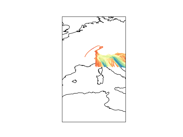
Plotting trajectories
To plot trajectories on top of a map, you can do the following:
>>> from dypy.lagranto import Tra
>>> trajs = Tra()
>>> trajs.load_netcdf(filename)
>>> m.plot_traj(trajs, 'QV', cm='Spectral',
                levels=np.arange(1, 12, 1))
Docstrings
-
class
dypy.plotting.plotting.Mapfigure(resolution='i', projection='cyl', domain=None, lon=None, lat=None, basemap=None, **kwargs)[source]¶ Class based on Basemap with additional functionality such as plot_trajectories
-
class
dypy.plotting.plotting.SkewT(ax, prange={'dp': 1.0, 'pbot': 1000.0, 'ptop': 100.0})[source]¶ Create a skewT-logP diagramm
-
es(T)[source]¶ Returns saturation vapor pressure (Pascal) at temperature T (Celsius) Formula 2.17 in Rogers&Yau
-
gamma_s(T, p)[source]¶ Calculates moist adiabatic lapse rate for T (Celsius) and p (Pa) Note: We calculate dT/dp, not dT/dz See formula 3.16 in Rogers&Yau for dT/dz, but this must be combined with the dry adiabatic lapse rate (gamma = g/cp) and the inverse of the hydrostatic equation (dz/dp = -RT/pg)
-